
In last article I talked about how to use only one simple spring force to set up a differential equation and solve it to give the dynamics of SHM, which is a typical projection of uniform circular motion. Forces that follow the Hook’s Law seem to be very special in real world. There are many forces which can be written in $F=-kx$, but I’m thinking about another “special” force, which are forces that is inversely proportional to the square of displacement, typically, gravitation and electrostatic attraction:
These two kind of forces seem to be the most special form of forces: because the solutions to differential equations describing motion due to these two forces automatically reduce to some beautiful expressions. In this article I’d like to share our investigation on the gravitational field, specifically, the motion of an object in a central gravitational force field. In last week’s physics club, we tried our best to understand all the quantitative calculations through simple calculus, and the following would be the proof of why the track of objects in a central gravitational force field would be a conic curve. The calculation itself is tedious, but it reveals how special the gravitational force is, or all the forces which are proportional to $\frac{1}{r^2}$
I also have a hand written version of the proof and it seems to be more intuitive. Of course it’s written in Chinese. Anybody who wants it can download directly from here.
Introduction to Conic Curves
You may have heard that the orbits of planets are elliptical, while the orbits of passing stars, such as the recently popular 3I Atlas, are hyperbolic. In general, these orbital shapes have a common name: conic sections. Why is that? We need to understand them.
Conic sections (or conic curves) are the curves obtained by intersecting a plane with a double-napped right circular cone. Depending on the angle of the plane, you get four distinct types: the circle, ellipse, parabola, and hyperbola.
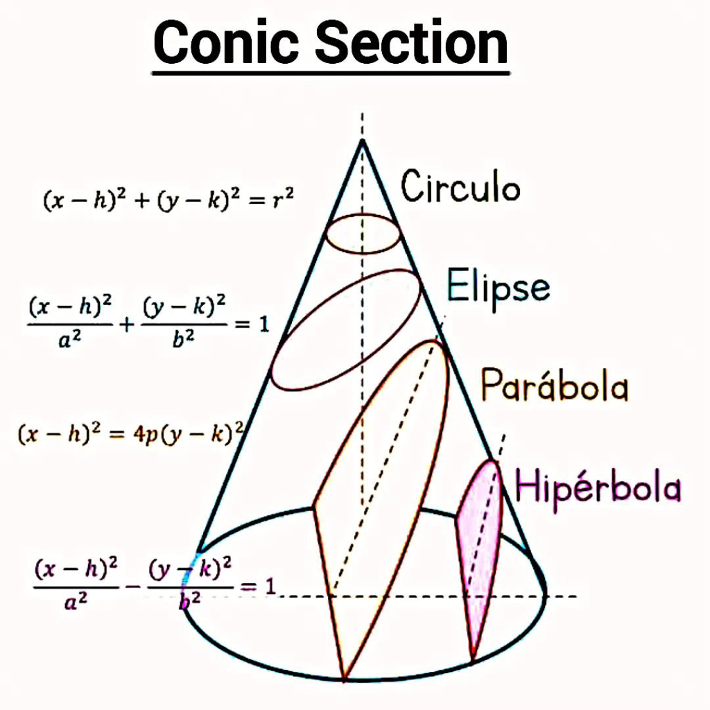
While they are often studied in Cartesian coordinates ($x, y$), their polar form is particularly elegant because it provides a single, unified equation for all conic sections.
The Unified Geometric Definition
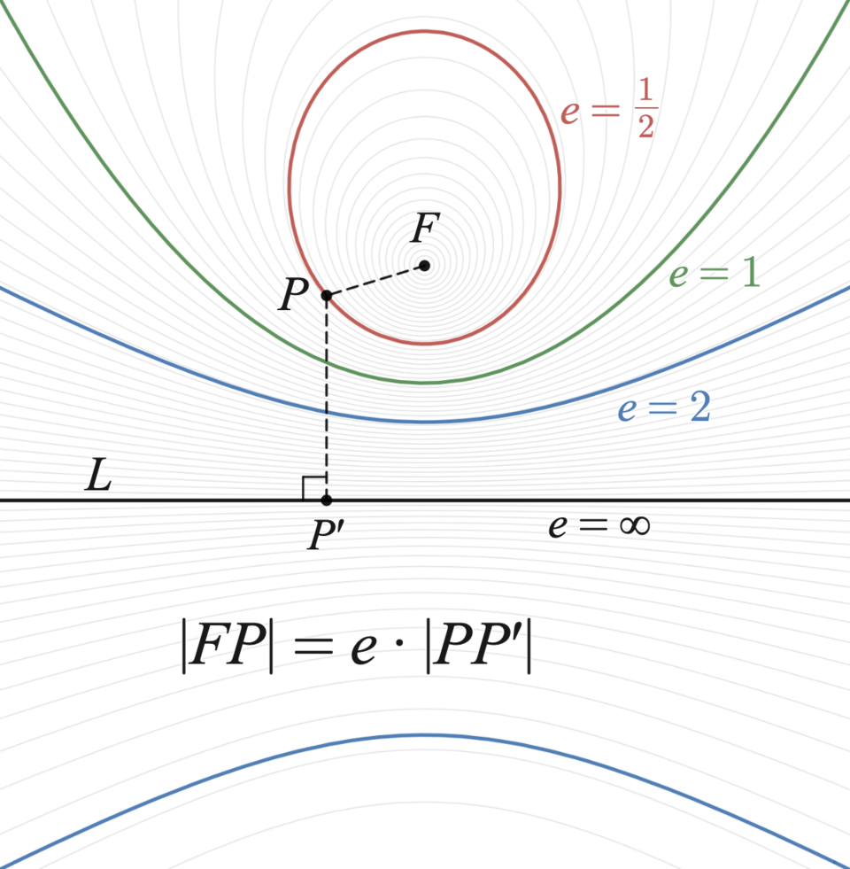
A conic section can be defined as the locus of all points $P$ such that the ratio of the distance from $P$ to a fixed point (the focus) to the distance from $P$ to a fixed line (the directrix) is a constant.
This constant ratio is called the eccentricity ($e$).
- Ellipse: $0 \le e < 1$ (A circle is a special case where $e = 0$)
- Parabola: $e = 1$
- Hyperbola: $e > 1$
The Polar Equation
In polar coordinates, we usually place the focus at the origin (pole). If the directrix is a vertical line at $x = d$, the general polar equation is:
$$r = \frac{ed}{1 + e \cos \theta}$$
Alternatively, it is often written using the semi-latus rectum ($l$), which is the distance from the focus to the curve along a line perpendicular to the major axis ($l = ed$):
$$r = \frac{l}{1 + e \cos \theta}$$
Variations in Orientation:
The form of the equation changes slightly depending on where the directrix is located relative to the focus:
- $1 + e \cos \theta$: Directrix is at $x = d$ (to the right of the focus).
- $1 – e \cos \theta$: Directrix is at $x = -d$ (to the left of the focus).
- $1 + e \sin \theta$: Directrix is at $y = d$ (above the focus).
- $1 – e \sin \theta$: Directrix is at $y = -d$ (below the focus).
Key Characteristics by Shape
The Ellipse ($0 < e < 1$)
The curve is closed. The polar equation describes an ellipse where the origin is one of the two foci. As $e$ approaches 0, the ellipse becomes more circular.
The Parabola ($e = 1$)
The denominator becomes $1 + \cos \theta$. When $\theta = \pi$, the denominator becomes 0, and $r$ goes to infinity. This reflects the “open” nature of the parabola.
The Hyperbola ($e > 1$)
The hyperbola has two branches. The polar equation $r = \frac{ed}{1 + e \cos \theta}$ produces both branches, though $r$ can take negative values for certain angles $\theta$ to represent the second branch.
The following Geogebra graph calculator embedded app helps with the understanding. You can change the value of $e$ using the slider and see what’s the changes.
A Seemingly Complete Proof
Here we come to the important part: proving that why object orbits the central force source with a track of conic curve. Like what we’ve doubted in the previous article, all of these statements should have mathematical foundations.
(Note: The following words are actually the English translation of my original hand written proof, with refined words.)
I. Constructing the Coordinate System and Force Analysis
First, constructing a coordinate system is an essential step. In a central force field like gravity, only one force exists—gravity itself—which can also be understood as the centripetal force. We construct a polar coordinate system with the central celestial body at the origin. Since the gravitational force points toward the center, its value is negative based on the definition and physical meaning of polar coordinates:
$$
F = – \frac{GMm}{r^2}
$$
However, we are missing the “other half” of the equation. The trajectory of the celestial body is not explicitly reflected in the expression for gravity. To bridge the gap between motion and force, we utilize Newton’s Second Law:
$$
F = – \frac{GMm}{r^2} = ma \implies a = – \frac{GM}{r^2}
$$
This will serve as our primary “springboard.” Let’s consider if any other known conditions have been overlooked: In a two-body system, the two bodies acting as a system are not subject to external forces, so the angular momentum of the system is conserved. Similarly, for the moving body in our problem, the torque exerted by the central body on it is zero.
Why? Because while there is a force in the radial direction, there is no component of force in the tangential direction:
$$
\tau = F \cdot \cos 90^\circ = 0
$$
(Note: Torque is zero because the force vector is parallel to the position vector). Therefore, angular momentum is conserved. I haven’t mathematically proven yet that the force is strictly perpendicular to the tangent of the trajectory—let’s leave that as a small “foreshadowing.”
II. Kinematic Derivation in Polar Coordinates
Based on the conservation of angular momentum, we write:
$$
L = m \omega r^2 = mvr
$$
However, $r$ has not yet been transformed into polar coordinate vectors.
The position vector is $\vec{r} = r \cdot \hat{r}$, where $r$ is the magnitude (distance) and $\hat{r}$ is the unit vector indicating the direction of $\vec{r}$. To find the velocity $\vec{v}$, we take the derivative of $\vec{r}$ with respect to time:
$$
\vec{v} = \dot{\vec{r}} = \dot{r}\hat{r} + r \frac{d\hat{r}}{dt} \quad \text{(Product Rule)}
$$
However, we don’t yet know the contribution of the derivative of the unit vector to the calculation. Let’s try to transform it:
$$
\hat{r} = \begin{pmatrix} \cos\theta \ \sin\theta \end{pmatrix} \quad \text{(From the definition of a unit vector)}
$$
$$
\frac{d\hat{r}}{dt} = \begin{pmatrix} -\sin\theta \cdot \dot{\theta} \ \cos\theta \cdot \dot{\theta} \end{pmatrix} = \dot{\theta} \begin{pmatrix} -\sin\theta \ \cos\theta \end{pmatrix}
$$
Notice that: $\begin{pmatrix} \cos\theta \ \sin\theta \end{pmatrix} \cdot \begin{pmatrix} -\sin\theta \ \cos\theta \end{pmatrix} = -\cos\theta \sin\theta + \sin\theta \cos\theta = 0$
The dot product of the two vectors is 0, meaning they are perpendicular.
In physical terms, if $\hat{r}$ is the direction of position, then the vector perpendicular to it represents the direction of rotation. As shown in the diagram, we define $\hat{\theta} = \begin{pmatrix} -\sin\theta \ \cos\theta \end{pmatrix}$, then:
$$
\frac{d\hat{r}}{dt} = \dot{\theta} \hat{\theta}, \quad \vec{v} = \dot{r}\hat{r} + r \dot{\theta} \hat{\theta}
$$
Continuing with the derivation, we need the acceleration:
$$
\vec{a} = \frac{d\vec{v}}{dt} = \ddot{r}\hat{r} + \dot{r} \frac{d\hat{r}}{dt} + \frac{d}{dt}(r \dot{\theta})\hat{\theta} + r \dot{\theta} \frac{d\hat{\theta}}{dt}
$$
$$
\vec{a} = \ddot{r}\hat{r} + \dot{r}\dot{\theta}\hat{\theta} + (\dot{r}\dot{\theta} + r\ddot{\theta})\hat{\theta} + r\dot{\theta} \frac{d\hat{\theta}}{dt}
$$
Just like before, let’s analyze $\hat{\theta}$:
$$
\hat{\theta} = \begin{pmatrix} -\sin\theta \ \cos\theta \end{pmatrix}, \quad \frac{d\hat{\theta}}{dt} = \begin{pmatrix} -\cos\theta \cdot \dot{\theta} \ -\sin\theta \cdot \dot{\theta} \end{pmatrix} = -\dot{\theta} \begin{pmatrix} \cos\theta \ \sin\theta \end{pmatrix} = -\dot{\theta} \hat{r}
$$
This simple substitution works because the components are exactly the negative of the original unit vector definitions. Therefore:
$$
\vec{a} = \ddot{r}\hat{r} + \dot{r}\dot{\theta}\hat{\theta} + (\dot{r}\dot{\theta} + r\ddot{\theta})\hat{\theta} – r\dot{\theta}^2\hat{r}
$$
$$
\vec{a} = (\ddot{r} – r\dot{\theta}^2)\hat{r} + (2\dot{r}\dot{\theta} + r\ddot{\theta})\hat{\theta}
$$
III. Angular Momentum and Specific Angular Momentum
When applying Newton’s Second Law, we are only concerned with the centripetal force—the force in the radial direction. Thus, only the radial acceleration $a_r = \ddot{r} – r\dot{\theta}^2$ is relevant. We can now construct the equation:
$$
\ddot{r} – r\dot{\theta}^2 = -\frac{GM}{r^2}
$$
However, we want to find an expression for $r(\theta)$. The presence of the time derivative $\ddot{r}$ complicates this by introducing the variable $t$. Since we haven’t used the conservation of angular momentum yet, let’s apply a transformation:
$$
L = mvr = m(r\dot{\theta})r = mr^2\dot{\theta} = \text{constant}
$$
The reason we replaced $v$ with $r\dot{\theta}$ is that in the context of angular momentum, we only care about the tangential component of velocity.
Since $m$ is constant, $r^2\dot{\theta} = \text{constant}$. We define this constant as the Specific Angular Momentum, $h = r^2\dot{\theta}$, which gives us $\dot{\theta} = \frac{h}{r^2}$. This allows us to eliminate $t$ and focus on the relationship between $r$ and $\theta$.
IV. The Binet Equation
Here, Newton (and later Binet) proposed a brilliant simplification: substitute $r$ with $u = 1/r$. I will discuss the reason for this at the end.
Thus, $\dot{\theta} = hu^2$. Substituting this into our equation:
$$
\ddot{r} – r(hu^2)^2 = \ddot{r} – r h^2 u^4 = -\frac{GM}{r^2}
$$
To find $\ddot{r}$, we first find $\dot{r}$. We use the chain rule to change the independent variable to $\theta$:
$$
\dot{r} = \frac{dr}{d\theta} \cdot \frac{d\theta}{dt} = \frac{d(1/u)}{d\theta} \cdot \dot{\theta} = -\frac{1}{u^2} \frac{du}{d\theta} \cdot hu^2 = -h \frac{du}{d\theta}
$$
$$
\ddot{r} = \frac{d}{dt}(\dot{r}) = \frac{d}{dt}(-h \frac{du}{d\theta})
$$
Since $h$ is a constant:
$$
\ddot{r} = -h \frac{d}{d\theta}\left(\frac{du}{d\theta}\right) \cdot \frac{d\theta}{dt} = -h \frac{d^2u}{d\theta^2} \cdot \dot{\theta} = -h \frac{d^2u}{d\theta^2} \cdot (hu^2) = -h^2 u^2 \frac{d^2u}{d\theta^2}
$$
Substituting this back into the original equation:
$$
-h^2 u^2 \frac{d^2u}{d\theta^2} – \frac{1}{u} (h^2 u^4) = -GM u^2$$
$$\Rightarrow -h^2 u^2 \left(\frac{d^2u}{d\theta^2} + u\right) = -GM u^2
$$
Dividing by $-h^2 u^2$:
$$
\frac{d^2u}{d\theta^2} + u = \frac{GM u^2}{h^2 u^2} = \frac{GM}{h^2}
$$
Which is:
$$
u” + u = \frac{GM}{h^2}
$$
This is a standard second-order non-homogeneous linear differential equation with constant coefficients. The general solution is:
$$
u(\theta) = \frac{GM}{h^2} + C \cos(\theta – \theta_0)
$$
V. Physical Meaning of the Orbit Equation
In this solution, $C$ is an integration constant related to the total energy of the system; $\theta_0$ is the phase constant, determined by the initial position of the orbit.
To get back to $r(\theta)$, we use $r = 1/u$:
$$
r(\theta) = \frac{1}{\frac{GM}{h^2} + C \cos(\theta – \theta_0)} = \frac{h^2 / GM}{1 + \frac{Ch^2}{GM} \cos(\theta – \theta_0)}
$$
This matches the polar equation for Conic Sections:
$$
r(\theta) = \frac{p}{1 + e \cos(\theta – \theta_0)}
$$
Where $p = \frac{h^2}{GM}$ (semi-latus rectum) and $e = \frac{Ch^2}{GM}$ (eccentricity).
To determine $C$: for such problems, the total mechanical energy $E$ is related to the eccentricity $e$ by:
$$
e = \sqrt{1 + \frac{2Eh^2}{G^2M^2}} = \frac{Ch^2}{GM}
$$
This allows us to solve for $C$.
VI. Conclusion and Reflection
We have proven that the trajectory of a body in a central gravitational field is a conic section. I haven’t explained why Newton used the $u = 1/r$ substitution yet. If we try to solve the differential equation directly for $r$ without the substitution, it becomes:
$$
r \cdot r” – 2(r’)^2 = r^2 – \frac{GM}{h^2}r^3
$$
This is significantly more difficult than $u” + u = \frac{GM}{h^2}$. In fact, the direct equation for $r$ cannot be easily solved using elementary functions.
We finally complete the proof! 🎉🎉🎉
It’s easy the find the inherent relationship between the two proofs we’ve made till now —- although I have to inform all of you that the Pi project doesn’t stop. Actually I’ve done a little experiment in our school’s lab for which I’m probably going to talk about in the next article.
The key method we’ve used in connecting forces and motions is differential equation. We find the equivalent values, set up an equation including differential forms of velocity and acceleration, and figure out how to solve them properly. Interestingly, the solutions to both complex equations are equivalent to the polar expressions of circle and conic sections respectively. You can try assuming the gravitational force is proportional to $1/r^3$ and you will probably find that the equation is really a mess and it is unable to be solved either (At least I don’t know how to).
So this is our extended part of physics club investigation. It’s hard for sure, but it reveals the mathematical relationship under the explicit presentation of physical phenomenon.
See more in Wikipedia’s introduction to Kepler’s Laws, including Newton’s explanation in his famous Philosophiæ Naturalis Principia Mathematica
https://en.wikipedia.org/wiki/Kepler%27s_laws_of_planetary_motion#Planetary_acceleration
Leave a Reply
You must be logged in to post a comment.